Goals of this Lesson:

1. Find the icon for the R Console Application (not RStudio)
2. Try out the R Console Application (not RStudio)

What tools do we need to use R in this course?

• • R Console Application
  • RStudio — the graphical interface for accessing the engine of R

We can run R via either of the above tools. But RStudio looks complicated. So our plan is to first learn R by using the R Console application first before we use RStudio.

What do you need to do for this lesson?

Step 1 — Download the R Console application and its graphical interface called RStudio. See the syllabus for download instructions.

Step 2 — Watch the video (scroll to the bottom of this page) which shows you how to do the R1 assignment. While the video demonstration uses a Mac, PC users should use a very similar screen layout in their R Console application.

Important !! — If you are a PC user, please read the following carefully:

If you are having great difficulty in creating your R script or saving your result in a text file because your R screen looks very different than that shown in the video, that probably means that you are not using the R Console application — you are using RStudio instead.

Here is how to find your R Console application on your PC:

https://www.course.cafe/math/lesson/running-r-console-application-on-pc/

Here is the video showing you how to do the R1 homework:

R1 – Try out the R Console Application

For PC:

Ch 1.1 and 1.2 of the documentation below also shows you how to interact with the R Console:

Instant-R

-END-

Goals of this lesson:

1) Create scatterplots:

plot()    pch()    col()

2) Generate correlation:

cor()

2) Generate linear regression result:

lm()

3) Draw a least-squares regression equation on your scatterplot:

abline()

Instructions

• Watch the following video:

Lesson 5 Linear Regression

• For the details on the “pch” argument, see the link:

http://www.sthda.com/english/wiki/r-plot-pch-symbols-the-different-point-shapes-available-in-r

• Here is a list of colors to choose from for the command col():

http://www.stat.columbia.edu/~tzheng/files/Rcolor.pdf

-END-

This homework set is based on Lesson 5 — Linear Regression. So you need to watch the video in Lesson 5  BEFORE you do this homework set.

I. Goals:

1) Create a scatterplot via the R commands:

plot ()   pch()   col()

2) Generate linear regression result:

lm()

3) Draw a least-squares regression equation on your scatterplot:

abline()

II. What to upload to Canvas for the R5 assigment?

You ONLY need to upload your R script to Canvas by the due date and time:

• • • R script (.R)

Important: What the grader and I will do is to run your .R script on our computer to generate the scatterplot. So make sure your .R script works!

The best way for you is to check if your script works or not is to do the following:

• • After you have uploaded your script to Canvas, log out of Canvas and then log back into Canvas. Download your .R script and run it on your RStudio to see if it works!

III. What to do for this assignment

• Create one .R script to generate a scatterplot with a linear regression line of two quantitative variables which are negatively-correlated.
  

Here are the Details:

1) Come up with two quantitative variables that are different than the ones shown in the video —

• • • Be creative! Don’t just copy my example. Come up with something DIFFERENT than the example shown in the demonstration — you will NOT receive full credit if your variables are TOO SIMILAR to mine — e.g. “tea” vs “awake time” or “soda” vs “sleep time” are TOO SIMILAR to my example!

• • • Your variables can be biology-related (but they don’t have to be).

• • • Label your variables clearly (e.g. calling your variable “school” or “season” is NOT clear enough)

• • • Come up with 8 pairs of observations with r negative but \(r \neq -1 \). That is, r should be negative but not equal to 1 exactly.

2) To receive full credits, your scatterplot needs to show the following:

• • • • 8 pairs of observations
      • a linear regression line
      • a title for the plot
        • you can but you don’t have to follow the format “…. vs ….” as shown in the video. You can come up with your own as long as it makes sense.
      • a label for the x-axis (include the unit of measurement)
      • a label for the y-axis (include the unit of measurement)

3) To receive full credits, your R script needs to satisfy the following:

• • • Show clearly how you use the commands below to generate a scatterplot with a linear regression line:
      • • plot()
        • pch() — you can choose any shape of data points
          
        • col() — you can choose any color of data points
          
        • lm()
        • abline ()

(No need to calculate correlation.)

• • • At the top of your R script, use # to:
      • Type your name AND

• • • • Type a sentence or two to state or describe your quantitative variables. Your variables can be biology-related (but they don’t have to be). The “negative” relationship should make sense  and the labeling should be specific enough.  If you are concerned whether the grader would understand the negative relationship between your variables, then just write a sentence or two in your script to explain.

• • • • It is optional to include other information such as assignment name, etc.

4) Upload the following item to Canvas by the due date and time.

• • • • R script (.R)

No need to upload your scatterplot.

-END-

This homework set is based on Lesson 3 — Boxplots. So you need to watch the video in Lesson 3 BEFORE you do this homework set.

I. Goal of this assignment:

Create side-by-side boxplots via the R command:

boxplot()

II. What to upload to Canvas for this R3 assigment?

You only need to upload ONE script only:

• • •  R script (.R)
      

(NO NEED to upload any result file or PDF)

Important: What the grader and I will do is to run your .R script on our computer to generate the boxplots. So make sure your .R script works!

The best way for you is to check if your script works or not is to do the following:

• • After you have uploaded your script to Canvas, log out of Canvas and then log back into Canvas.  Download your .R script and run it on your R Console to see if it works!

III.  What to do for this assignment

Create one .R script to satisfy the following requirements:

(There is only one question in this assignment.)

1)  Come up with a quantitative variable with two sets of data.

• • • Be creative! Don’t just copy my example.  Come up with something DIFFERENT than the example shown in the demonstration —  you will NOT receive full credit if your variable and conditions are TOO SIMILAR to mine — e.g. “plants grown under two weather conditions” or “seeds grown under two soil conditions” are TOO SIMILAR to my example!

• • •  Each set of data should consists of 10 to 20 data points.

2) Construct two boxplots for the two sets of data on ONE single scale.

• • • That is, you create side-by-side boxplots on one single scale —no credit will be given if this requirement is not satisfied.

• • • Your boxplots can be vertical or horizontal. (But don’t do both!)

3) At the top of your R script, use # to

• • • type your name AND

• • • type a sentence or two to describe your quantitative variable and the two conditions. Your variable can be biology-related (but they don’t have to be).  Just make sure that your variable and conditions makes sense.

• • • It is optional to include other information such as assignment name, etc.

4) To receive full credit, make sure your diagram of boxplots shows the following:

• • • each boxplot has one outlier (it can be a high or low outlier)
    • a chart title for the entire diagram
    • labels for the horizontal and vertical axes (include unit of measurement for one of the axes)
    • a label for each boxplot

5) Upload your .R script to Canvas by the due date and time. No need to upload your boxplots pdf.

The video shows you how to save your boxplots diagram as a PDF so that you have a record for yourself of what you have done. However, you DO NOT need to upload your PDF into Canvas.

-END-

I. Goals of this Lesson:

1) Create side-by-side boxplots via the R command (scroll to the bottom of the page for details):

boxplot()

2) Learn the R command to remove all objects:

rm(list=ls())

(Scroll to the bottom of the page for the commands to clear the screen.)

II.Watch the video to learn how to create boxplots:

Lesson 3 — Boxplots

III. Here are the arguments (inputs) to include in the command boxplot():

names               Group labels which will be printed under each boxpot

xlab                   Label for the x axis

ylab                   Label for the y axis

main                 Title for the entire diagram

col                     Colors for the boxplots (see below for more details)

IV. If you want to do horizontal boxplots, include the following argument (you also need to make sure your x label and y label make sense).

horizontal         TRUE

V. Here is a list of colors in R:

http://www.stat.columbia.edu/~tzheng/files/Rcolor.pdf

VI. To clear your screen in the R Console:

To clear the screen in Mac, type command + option + L

To clear the screen in Windows, type control + L

-END-

Goals of this lesson:

1) Learn to use RStudio

2) Create histograms via the R command:

hist()

Installing and Starting RStudio

Notice that the RStudio and R Console applications have different icons:

If you haven’t installed RStudio, see the download instructions on the syllabus for details.

If you use a PC, please note that RStudio has the same layout on both Macs and PCs. If you find your screen layout very different than that shown in the video, that means that you are not using the RStudio application.

To find where the RStudio is on your PC and what the screen layout looks like, watch the following video starting from the time-mark of 3:00:

https://www.youtube.com/watch?v=GAGUDL-4aVw

Lesson video

Watch the following video and do your R4 assignment. While the video demonstration below uses a Mac, both PC and Mac users will see a avery similar screen layout in R.

Lesson 4— RStudio & Histogram

Here are the arguments (inputs) to include in the command hist():

name of vector — name of object which you have created to store the data values

main — Title for the plot

xlab — Label for the x axis

Don’t forget to separate the arguments with comma!

-END-

This homework set is based on Lesson 4 — RStudio & Histograms. So you need to watch the video in Lesson 4 BEFORE you do this homework set.

I. Goals of this assignment:

1) Run R in RStudio

2) Create a histogram via the R command:

hist()

3) Understand the relationship between data skewedness and shape of histogram.

II. What to upload to Canvas for the R4 assigment?

Upload the following 2 items to Canvas by the due date and time:

• • • RStudio screenshot (.pdf)
    • R script (.R)

Important: What the grader and I will do is to run your .R script on our computer to generate the boxplots. So make sure your .R script works!

The best way for you is to check if your script works or not is to do the following:

• • After you have uploaded your script to Canvas, log out of Canvas and then log back into Canvas. Download your .R script and run it on your R Console to see if it works!

III.  What to do for this assignment

• Create one .R script to generate a left-skewed histogram (see details below)

AND

• Take a screenshot of your RStudio windows and convert it to PDF

Here are the Details:

1) Come up with a quantitative variable that is different than the one shown in the video —

• • • Be creative! Don’t just copy my example.  Come up with something DIFFERENT than the example shown in the demonstration —  you will NOT receive full credit if your variable is TOO SIMILAR to mine — e.g. “monthly rainfall amount” or “annual rainfall amount” are TOO SIMILAR to my example!

• • • Your variable can be biology-related (but they don’t have to be).

• • • Label your variable clearly (e.g. calling your variable “school” or “season” is NOT clear enough)

• • • Make up between 10 to 40 observations so that the histogram is roughly skewed to the left. Repeated data values (observations) are allowed.

2) Your histogram needs to satisfy the following:

• • • the shape should be roughly skewed to the left
      

• • • the histogram should have a minimum of 4 bars but no more than 12 bars

• • • a chart title for the histogram

• • • a label for the x-axis (include the unit of measurement)

3) At the top of your R script, use # to:

• • • Type your name AND

• • • Type a sentence or two to describe your quantitative variable.  Your variable can be biology-related (but they don’t have to be).  Just make sure that your variable makes sense and the labeling is specific enough.

• • • It is optional to include other information such as assignment name, etc.

4) Take a screenshot of your RStudio windows and convert that screenshot to a PDF.

• • • The screenshot PDF of your RStudio session should show all 4 windows —

• • • • Script window showing your R commands

• • • • Console window showing certain commands being executed (it’s OK if your Console window shows errors).

• • • • Environment window showing your vector (object)

• • • • Plot window showing your histogram

5) Upload the following 2 items to Canvas by the due date and time.

• • • • RStudio screenshot (.pdf)
      • R script (.R)

No need to upload your histogram plot.

The video shows you how to save your histogram plot as a PDF because it is always necessary to do when for a research project or research article. However, for this assignment you DO NOT need to upload the histogram plot into Canvas.

-END-

Goals:

• Create an R script to run basic commands to obtain mean, median, standard deviation and summary for data sets.

• Acquire a sense of the size of the mean, median and how “spread out“ a small set of observations are. For example, when we say the standard deviation is 2, how spread out do we expect our data values are around the center and from each other? Of course, we can always easily calculate the mean, median and standard deviation by our calculator or R. But it is important to get an intuitive feel for these measures.

Instructions

Please follow the instructions below carefully as that’s how the grader grades your assignment. Computer work is all about details!

1) This homework set is based on Lesson 2 — Basic Commands and scripts. So you need to watch the video in Lesson 2 BEFORE you do this homework set.

2) There are altogether 5 questions in this homework.

• • Create a R script to type your R commands for the 5 questions below.

• • At the top of your R script, use # to type your name (it is optional to include other information such as assignment name, etc).

• • For each question, use # to type the question number.

• • Upload the R script (with the file extension .R) to Canvas. Canvas will only accept a file with the .R extension. That’s ALL you need to upload to Canvas for this assignment — you do NOT need to upload any .txt file.

• • Make sure your R script works because the grader and I will run your R script and grade the results generated from your R script.

• • Scroll to the bottom of this page to see what your .R script should look like.

Here are the 5 questions in this assignment:

1) Create an object (a vector) with the following properties:

• • • 3 different numbers such that the mean is between 11 and 13 inclusively (that is, the mean can be 11 and 13 if you wish)
    • the mean does NOT have the same value as any of the numbers in your object
    • you can name the object (vector) anything you want

Run the mean () command in your .R script.

2) Create an object (a vector) with the following properties:

• • • 5 different numbers such that the median is between 20 and 25 inclusively
    • you can name the object (vector) anything you want

Run the median () command in your .R script.

3) Create an object (a vector) with the following properties:

• • • 5 different numbers between 10 and 90 inclusively
    • the mean is smaller than the median
    • you can name the object (vector) anything you want

Run the summary () command in your .R script.

4) Create an object (a vector) with the following properties:

• • • 5 different numbers between 10 and 90 inclusively
    • the standard deviation of the 5 numbers is between 1 to 3 inclusively
    • you can name the object (vector) anything you want

Show the sd () command in your .R script.

5) Create an object (a vector) with the following properties:

• • • 5 different numbers between 10 and 90 inclusively
    • the standard deviation of the 5 numbers is between 6 to 10 inclusively
    • you can name the object (vector) anything you want

Show the sd () command in your .R script.

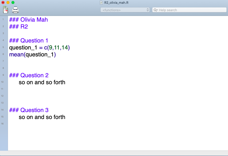
Here is what your .R script should look like:

-END-

Goals of this Lesson:

• Use the basic commands:

c( ) ls( ) rm( ) mean( ) median( ) sd( ) summary( )

• Create a R script

1. 1. 1. Use # to write comments.
      2. Execute commands via an R script (a file with file extension .R).

Instructions

1.  Watch the following video and do your R2 assignment. While the video demonstration below uses a Mac, both PC and Mac users will see a very similar screen layout in the R Console.

R2 — Basic commands & scripts

           (Note: You only need to upload the .R script to Canvas, not the .txt file.)

2)  If you notice that your screen layout looks very different than that shown in the video, that probably means that you are using the RStudio instead of the R Console.

For PC users, in case you cannot find the menu option to save your script, please watch the following video at the timestamp 6:29 —

https://www.youtube.com/watch?v=Q3NxsSRxKek

 3) If the file extension .R is not shown when you are saving the file in the R Console, it’s probably because your desktop is not set to show file extensions.

Here is how to set your desktop to show file extension:

For Mac:

https://support.apple.com/guide/mac-help/show-or-hide-filename-extensions-on-mac-mchlp2304/mac

For Window 10 on PC:

https://vtcri.kayako.com/article/296-view-file-extensions-windows-10

-END-

Instructions

Please follow the instructions below carefully as that’s how the grader grades your assignment. Computer work is all about details!

1) This homework set is based on Lesson 1 — Try out the R Console Application. So you need to watch the video in Lesson 1 BEFORE you do this homework set.

2) Here is the what you need to do for this assignment:

In the video, I typed three arithmetic operations: 2 + 3, 6*10 and 7/3.

— Now, what you need to do is to come up with your own three arithmetic operations (addition, multiplication and division). For example, you can type 101 +7, 60*2 or 55/9.

— You do NOT need to clear your screen in doing your assignment. (For some of you, you might see a bunch of text displayed on the screen after your three arithmetic operations. That’s fine. Just leave it there. See irrevelant_text.

— Then save your results in a .txt file (as shown in the video).

— Submit your .txt file to Canvas before the due date.

3) Regarding the .txt file:

For PC:

-END-