Physical History
Economic Bubbles
By Administrator
First published on May 17, 2019. Last updated on January 19, 2021.
Here we discuss economic regimes, more commonly known as “bubbles”.
Economic Flows
Food and mineral flows also represent economic flows. So do transfers from one group to another, such as from parent to children, workers to retirees, exporter to importer. Flows often work at least two ways. For example, goods and services flow from an exporter while money flows from an importer. Many trade partners engage in both importing and exporting with each other.
Financial Flows
Economic flows can be abstracted into financial flows, such as an annual market demand or income. An example of a steady income flow is called an annuity.
Direct Logistic or Gaussian Approach
It is traditional to model growth by one of two types of curves, the pure exponential growth curve or the logistic growth curve. Since most new business plan for three to five years, this is a reasonable approach.
All things end sooner or later, so it might make more sense to model growth with a Gaussian or Maxwell-Boltzmann distribution. However, most businesses don’t like to plan for a downturn. Yet for particular products or businesses in industries where the typical lifetime may only be a few year or a single season, either of these curves may be superior to the pure exponential or logistic approaches.
Beginning Point
None of these approaches has a clear beginning point, mathematically speaking. The pure exponential, logistic and Maxwell-Boltzmann curves can arbitrarily be assigned a beginning point without too much thought.
The Gaussian curve can prove more challenging to assign a beginning point. A fair approach is to initially establish a pure exponential growth curve, then later fit a Gaussian to that curve.
Pure Exponential Growth Phase
Sometimes it is hard to determine the parameters soon enough to make useful forecasts. Yet there are ways to handle this, although they are imperfect. However, if a business has a great product, and there is strong demand for it, the question is how quickly can the business expand to meet that demand? If the expansion cost and resultant speed can be calculated, then a model exponential growth curve can be generated, assuming that the business will expand as quickly as possible. Also assumed is that the growth of the business at a particular time will be proportional to its size at that time. If the business can only expand linearly, then a linear model must be generated.
Leveling or Decline Phases
Eventually, limiting factors will level off growth and even cause a decline in business. A logistics curve is appropriate for a product or business that will have relatively long-term, stable sales, such as a popular soft drink. For products that will have a known or likely decrease, a Gaussian or Maxwell-Boltzmann curve can model both the growth and decline.
Efficiency Approach
A more fundamental approach is to use efficiency data for modeling. This approach can work better if there are similar cases available for comparison so that reasonable parameters for reproduction costs and efficiency can be proposed at an early phase so that reasonable forecasts might be possible. This approach is similar to modeling a single historical regime.
Two Places to Begin—Relation to Supply and Demand
There are two placed to begin using the efficiency approach. One way is to determine the total lifetime sales for the product or business. (Take the raw value, not the Net Present Value-discounted value). If you can then determine what the peak sales amount will be, and the beginning and end dates of the business, you can treat efficiency as a linearly decreasing quantity (this is not entirely accurate, particularly for the beginning and end of the lifecycle, but can be a reasonable approximation).
A perhaps better, but more complicated way is to first model demand for the product (in terms of a series of classical economic demand curves over time). Then determine a series of classic supply curves over time. This will tell you the sales revenue and volume over time. The trick is to use fast entropy and thermodynamic efficiency to model how the supply and demand curves will change over time. Fast entropy will cause the quantity supply curve to fall: as the business develops, the business will likely increase production capacity, so that it can afford to sell more at a lower per unit price.
However, as time goes on, the demand curve will also fall due to growth leveling off or falling as the market becomes saturated. It is also possible, that there will be limits to how much production can grow is a required resource becomes scarcer (and thus expensive), so that the supply curve can only fall so far. These events represent decreasing thermodynamic efficiency. Thermodynamic efficiency should be differentiated from empirical efficiency, which may be due to such factors as economies of scale. In fact, it is often falling thermodynamic efficiency that required increased economies of scale to meet demand at sufficiently low prices. This is one reason why there is often consolidation in maturing industries.
Modeling Macroeconomic Business Cycles
It is possible to use this approach to model entire macro economic business cycles. (Despite their name, these cycles are really thermodynamic bubbles).
US Adjusted GNP Example
Figure below shows US adjusted GNP for 1993-2013 (the scale is nominal), a litter “sizzle” plot of the U.S. economy during that period. Long-term trends have been stripped out of the data. The figure shows the dot com bubble peaking around 2001 and the housing bubble peaking around 2006. These bubbles are not just random occurrences, for they share a similar structure. There is an underlying thermodynamic potential. . An engine of GNP growth forms to bridge that potential, such as firms that can create or take advantage of new computing technology or a relaxation of banking standards. At the beginning of the bubble, the potential is high, so that exploitation can take place at a high thermodynamic efficiency. However, as potential is consumed, the amount potential decreases, so efficiency necessarily drops. At the same time, old firms are expanding and new firms are being formed, resulting an increasing amount of heat engines” to consume potential.
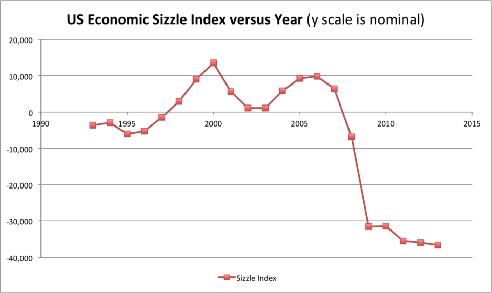
US Economy Sizzle Index 1993-2013
Once formed, these firm heat engines remain “hungry”. They need to consume potential to survive and they very badly want to survive and grow. So they keep growing, even though potential is decreasing. Eventually, the potential (and therefore thermodynamic efficiency) drops so low and there are so many heat engines, that most of the heat engines can no longer support themselves. Chances are, industry overshoot has occurred (i.e. formation of too many hungry heat engines), and a crash occurs. This cycle usually repeats itself for each macroeconomic business cycle bubble, although the chief industries involved may vary among bubbles. The bubble itself apparently increases overall entropy production of a society, which is consistent with the principle of fast entropy.